Generate Small Area Estimates

Primary SAE prediction function in hbsaems (supersedes deprecated hbsae). Computes area-level posterior predictive means, standard deviations, and relative standard errors (RSE).

Usage

sae_predict(
  model,
  newdata = NULL,
  predict_type = c("epred", "response", "linpred", "proportion"),
  ...
)

Arguments

model

An hbmfit or brmsfit object.

newdata

Optional new data.frame for prediction at unsampled areas. If NULL (default), the original data are used.

predict_type

Character; the posterior quantity to summarise. One of:

"epred" (default, new in 1.1.0)

Posterior of the area mean \(\theta_i = E[y_i \mid x_i, u_i]\) via posterior_epred. This is the correct SAE target; its per-area SD excludes observation-level likelihood variance.

"response"

Posterior predictive of a NEW observation \(\tilde y_i\) via posterior_predict. This was the 1.0.x behaviour; use it when predicting fresh observations or aggregate counts where observation variability is wanted.

"linpred"

Linear predictor on the response scale via posterior_linpred with transform = TRUE. For a binomial family this is the area proportion \(p_i\).

"proportion" (new in 1.1.0)

The area proportion \(p_i\). For a binomial family this divides the expected count by the trials (\(E[y_i]/n_i\)), giving a quantity comparable across areas with different sample sizes; identical to "linpred". For non-binomial families it equals "epred".

Binomial note. For a binomial family posterior_epred() returns the expected count \(n_i p_i\), which is not comparable across areas with unequal \(n_i\). The SAE target is normally the proportion \(p_i\), so predict_type = "epred" on a binomial model automatically returns \(p_i\) (with a warning); use "response" for the expected count, or "proportion" to request the proportion explicitly.

...

Additional arguments forwarded to posterior_predict (e.g.\ ndraws, re_formula).

Value

An hbsae_results object with components:

result_table

A data.frame with columns Prediction, SD, RSE_percent.

rse_model

Mean of RSE_percent across all areas.

pred

Numeric vector of point predictions (= result_table$Prediction).

Details

For each area \(i = 1, \ldots, n\), the function computes $$\widehat{y}_i = \frac{1}{S} \sum_{s=1}^{S} y_{i}^{(s)}, \qquad \widehat{\mathrm{sd}}_i^2 = \frac{1}{S - 1} \sum_{s=1}^{S} \left( y_{i}^{(s)} - \widehat{y}_i \right)^2,$$ where \(\theta_{i}^{(s)}\) are posterior draws of the area-mean target (predict_type = "epred", the default) – or of a new observation \(y_i^{(s)}\) when predict_type = "response" – and \(S\) is the number of draws. The relative standard error is \(\mathrm{RSE}_i = 100 \cdot |\widehat{\mathrm{sd}}_i / \widehat{y}_i|\).

See also

sae_aggregate, model_average, sae_transform, sae_scale, sae_filter

Examples

# \donttest{
library(hbsaems)
library(brms)
data("data_fhnorm")
model <- hbm(
  formula = brms::bf(y ~ x1 + x2 + x3),
  data    = data_fhnorm,
  chains = 4, iter = 2000, warmup = 1000, cores = 1,
  seed = 123, refresh = 0
)
#> Warning: Model fitted without any area-level random effects.
#>   This is unusual for Small Area Estimation: the standard Fay-Herriot model assumes u_i ~ N(0, sigma_u^2) per area, so estimates from a purely fixed-effects model will not borrow strength across areas.
#>   Consider one of:
#>     re = ~ (1 | area_id)                                     # IID area RE
#>     spatial_var = 'area_id', spatial_model = 'car', M = W    # CAR spatial RE
#>     spatial_var = 'area_id', spatial_model = 'sar', M = W    # SAR spatial RE
#>   If a fixed-effects-only baseline is intentional, you can suppress this warning with `suppressWarnings()`.
#> Compiling Stan program...
#> Start sampling
est <- sae_predict(model)
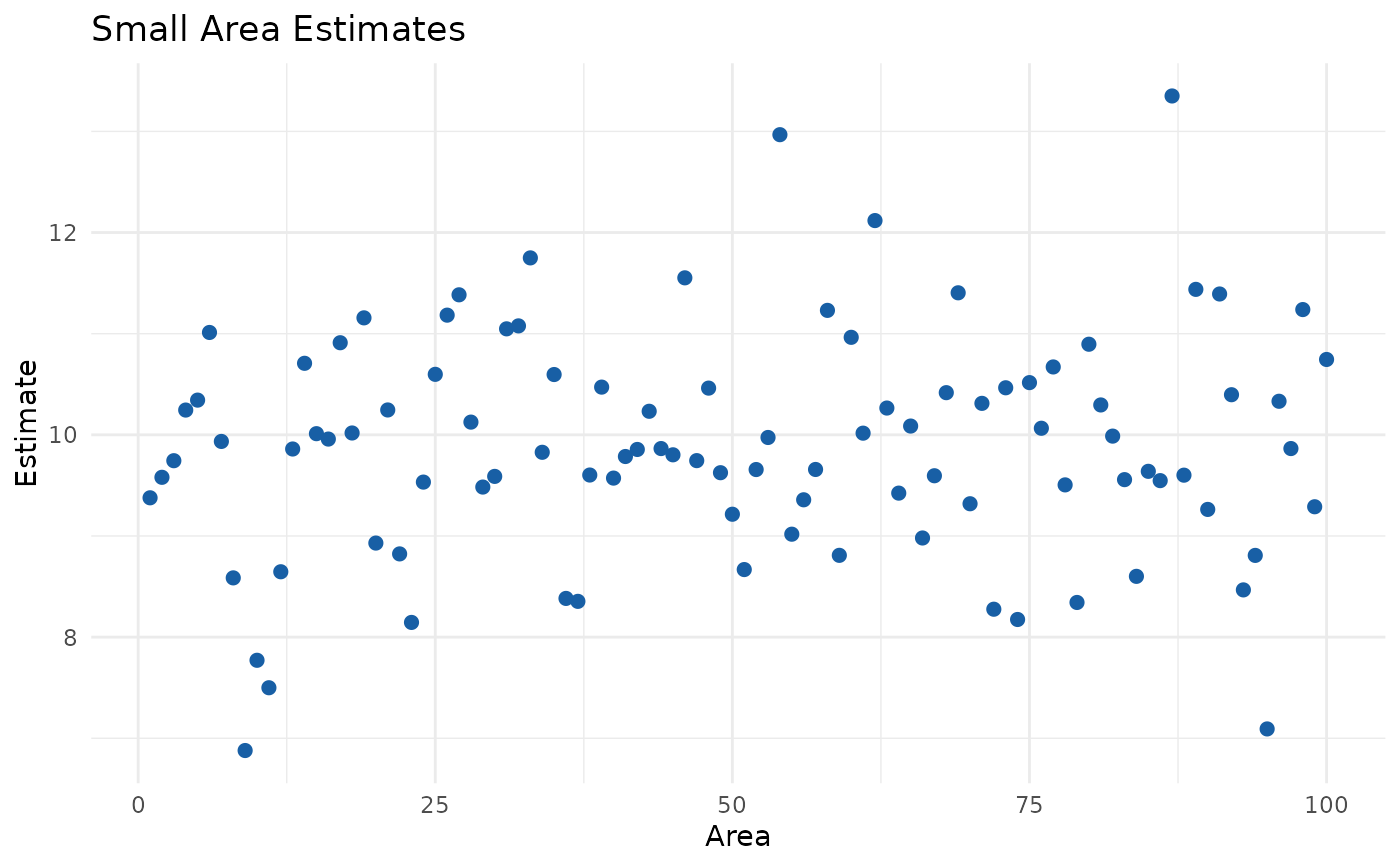
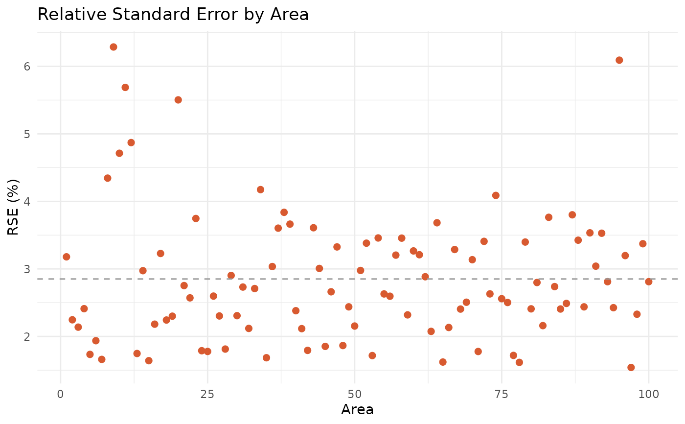
summary(est)
#> 
#> ===== Small Area Estimation Summary =====
#> 
#> Areas       : 100 
#> Overall RSE : 2.85 %
#> 
#> Predictions:
#>    Min. 1st Qu.  Median    Mean 3rd Qu.    Max. 
#>   6.879   9.348   9.862   9.892  10.483  13.350 
#> 
#> RSE by area:
#>    Min. 1st Qu.  Median    Mean 3rd Qu.    Max. 
#>   1.541   2.176   2.646   2.851   3.375   6.286 
plot(est, type = "predictions")

plot(est, type = "uncertainty")

# }