Generates prior predictive samples from a model fit with
sample_prior = "only" and compares them to the observed data.
This is the primary prior-check function (supersedes the deprecated
hbpc).
Arguments
- model
An
hbmfitorbrmsfitobject fit withsample_prior = "only"(seehbm).- data
A
data.framecontaining the response variable. Optional since 1.1.0: ifNULL(default) the data frame stored on the fitted model is used.- response_var
Character scalar naming the response column. Optional since 1.1.0: if
NULL(default) it is determined from the model formula's left-hand side.- ndraws_ppc
Integer. Number of prior predictive draws to overlay on the plot (default
50).- ...
Currently unused; reserved for future extensions.
Value
An hbpc_results object with components:
prior_predictive_plotA
ggplotfrompp_check, orNULLif it could not be generated.prior_drawsA draws matrix from
posterior_predictsizedndraws_ppc \times nrow(data).observedThe observed response vector.
Details
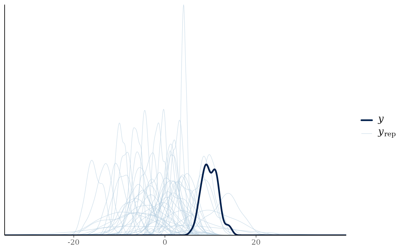
The prior predictive distribution is $$p(y_{\text{rep}}) = \int p(y_{\text{rep}} \mid \theta)\, p(\theta) \, \mathrm{d}\theta,$$ the marginal distribution of new data under the prior alone. Comparing it to the observed data is a fast sanity check: if the prior predictive places no mass anywhere near the data, the priors are likely too tight or in the wrong location.
Automatic argument detection (1.1.0)
When data is omitted it is taken from model$data (the model
frame stored on the fit). When response_var is omitted it is read
from the model formula via brmsterms; if the formula
has no left-hand side (so no response can be determined), an error is
raised asking the caller to supply response_var explicitly.
Examples
# \donttest{
library(hbsaems)
library(brms)
data("data_fhnorm")
model_prior <- hbm(
formula = brms::bf(y ~ x1 + x2 + x3),
data = data_fhnorm,
sample_prior = "only",
prior = c(
brms::prior(normal(0, 1), class = "b"),
brms::prior(normal(0, 5), class = "Intercept")
),
chains = 4, iter = 2000, warmup = 1000, cores = 1,
seed = 42, refresh = 0
)
#> Warning: Model fitted without any area-level random effects.
#> This is unusual for Small Area Estimation: the standard Fay-Herriot model assumes u_i ~ N(0, sigma_u^2) per area, so estimates from a purely fixed-effects model will not borrow strength across areas.
#> Consider one of:
#> re = ~ (1 | area_id) # IID area RE
#> spatial_var = 'area_id', spatial_model = 'car', M = W # CAR spatial RE
#> spatial_var = 'area_id', spatial_model = 'sar', M = W # SAR spatial RE
#> If a fixed-effects-only baseline is intentional, you can suppress this warning with `suppressWarnings()`.
#> Compiling Stan program...
#> Start sampling
# Explicit (as before):
pc <- prior_check(model_prior, data = data_fhnorm, response_var = "y")
# New in 1.1.0 -- data and response auto-detected from the model:
pc <- prior_check(model_prior)
print(pc)
#>
#> Prior Predictive Check [hbpc_results]
#> ----------------------------------------
#> Prior draws : 50 x 100
#> Observations : 100
#>
plot(pc)
 # }
# }